mcm
MCM
Introduction
The mcm function is a simple tool for analyzed different metrics from a confusion matrix. Can be very useful to analyze the performance of a binary classification model.
This function depends of pandas and the function confusion_matrix from sklearn.metrics. With confusion_matrix the True Negative (TN) cases, True Positive (TP) cases, False Negative (FN) cases and False Positive (FP cases) are calculated.
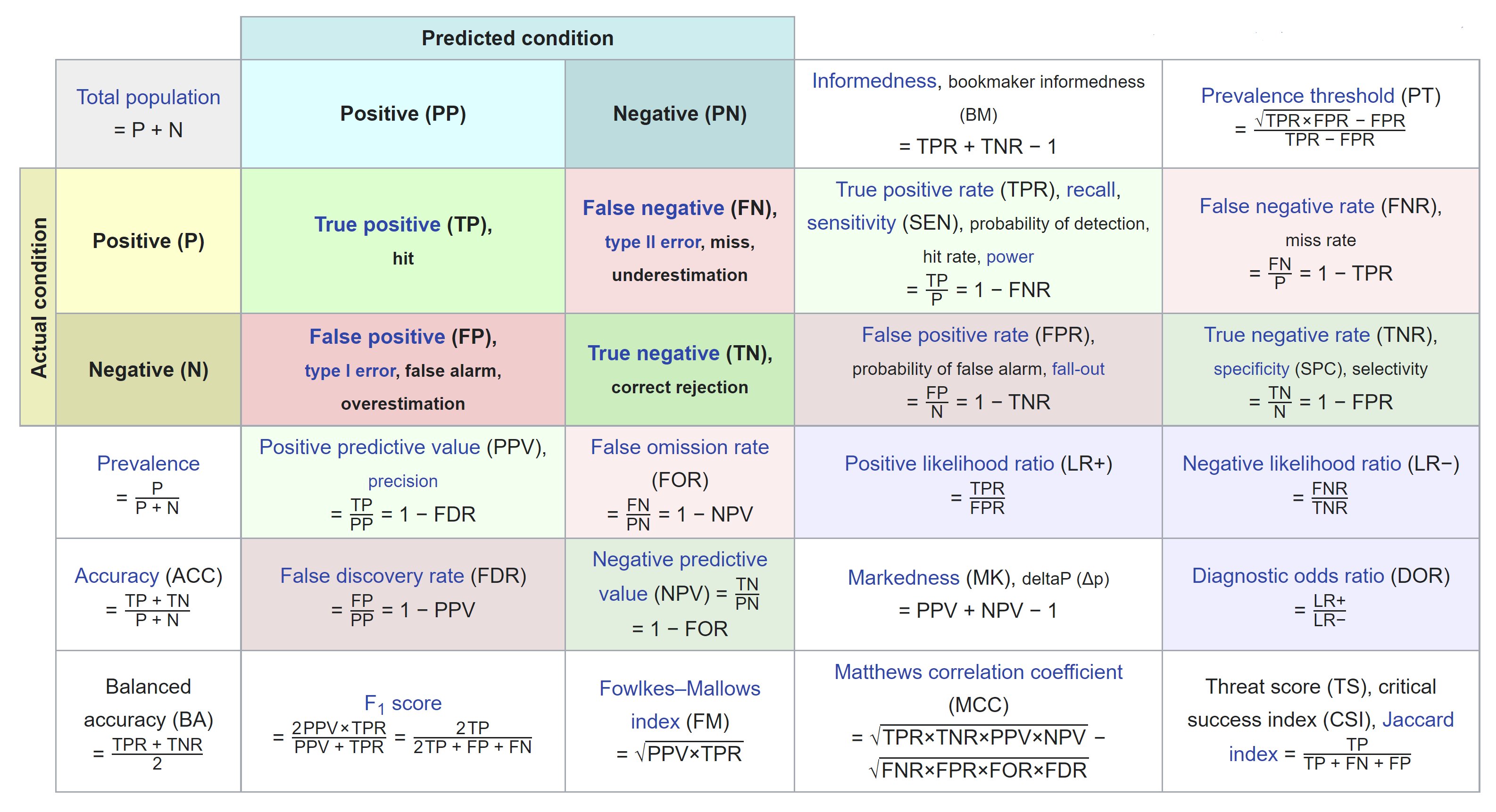
The following table categorizes predicted and actual conditions into four fundamental outcomes: True Positives (TP), True Negatives (TN), False Positives (FP), and False Negatives (FN).
Here are some key sections and their purpose:
-
Basic Definitions:
- Defines TP, TN, FP, and FN, which are the basic building blocks for further calculations.
-
Rates and Values:
- True Positive Rate (TPR): Also known as recall or sensitivity, measures the proportion of actual positives correctly identified.
- False Positive Rate (FPR): Measures the proportion of actual negatives incorrectly identified as positive.
- True Negative Rate (TNR): Also known as specificity, measures the proportion of actual negatives correctly identified.
- False Negative Rate (FNR): Measures the proportion of actual positives that were not detected.
-
Predictive Values:
- Positive Predictive Value (PPV): Also known as precision, measures the proportion of predicted positives that are true positives.
- Negative Predictive Value (NPV): Measures the proportion of predicted negatives that are true negatives.
-
Composite Metrics:
- Accuracy (ACC): Overall effectiveness of the classifier, measuring the proportion of true results (both true positives and true negatives).
- F1 Score: Harmonic mean of precision and recall, balancing the two metrics.
- Matthews Correlation Coefficient (MCC): Measures the quality of binary classifications, robust even if classes are of very different sizes.
-
Advanced Ratios:
- Likelihood Ratios (LR+ and LR-): Measure how much a test result will change the odds of having a condition.
- Diagnostic Odds Ratio (DOR): Ratio of the odds of the test being positive if the subject has a condition versus if the subject does not have the condition.
The table is designed to help in the interpretation of test results, particularly in the context of diagnostic tests or in the performance evaluation of classification algorithms. Each metric provides a different insight into the accuracy and reliability of the test or model, allowing practitioners to assess its effectiveness comprehensively.
The table below illustrates the confusion matrix used in our analysis. This matrix visualizes the performance of the classification algorithm, highlighting the true positives, true negatives, false positives, and false negatives. Understanding these values is crucial for evaluating the accuracy and reliability of our model.

The following Python code demonstrates how to generate a confusion matrix using the pandas and sklearn.metrics libraries. This matrix is pivotal for calculating various performance metrics, such as precision and recall, which help further assess the effectiveness of the model.
import pandas as pd
from sklearn.metrics import confusion_matrix
?confusion_matrix
Compute confusion matrix to evaluate the accuracy of a classification.

By definition a confusion matrix :math:`C` is such that :math:`C_{i, j}`
is equal to the number of observations known to be in group :math:`i` and
predicted to be in group :math:`j`.

Thus in binary classification, the count of true negatives is
:math:`C_{0,0}`, false negatives is :math:`C_{1,0}`, true positives is
:math:`C_{1,1}` and false positives is :math:`C_{0,1}`.

Read more in the :ref:`User Guide <confusion_matrix>`.

Parameters
----------
y_true : array-like of shape (n_samples,)
    Ground truth (correct) target values.

y_pred : array-like of shape (n_samples,)
    Estimated targets as returned by a classifier.

labels : array-like of shape (n_classes), default=None
    List of labels to index the matrix. This may be used to reorder
    or select a subset of labels.
    If ``None`` is given, those that appear at least once
    in ``y_true`` or ``y_pred`` are used in sorted order.

sample_weight : array-like of shape (n_samples,), default=None
    Sample weights.

normalize : {'true', 'pred', 'all'}, default=None
    Normalizes confusion matrix over the true (rows), predicted (columns)
    conditions or all the population. If None, confusion matrix will not be
    normalized.

Returns
-------
C : ndarray of shape (n_classes, n_classes)
    Confusion matrix.

References
----------
.. [1] `Wikipedia entry for the Confusion matrix
       <https://en.wikipedia.org/wiki/Confusion_matrix>`_
       (Wikipedia and other references may use a different
       convention for axes)

Examples
--------
>>> from sklearn.metrics import confusion_matrix
>>> y_true = [2, 0, 2, 2, 0, 1]
>>> y_pred = [0, 0, 2, 2, 0, 2]
>>> confusion_matrix(y_true, y_pred)
array([[2, 0, 0],
       [0, 0, 1],
       [1, 0, 2]])

>>> y_true = ["cat", "ant", "cat", "cat", "ant", "bird"]
>>> y_pred = ["ant", "ant", "cat", "cat", "ant", "cat"]
>>> confusion_matrix(y_true, y_pred, labels=["ant", "bird", "cat"])
array([[2, 0, 0],
       [0, 0, 1],
       [1, 0, 2]])

In the binary case, we can extract true positives, etc as follows:

>>> tn, fp, fn, tp = confusion_matrix([0, 1, 0, 1], [1, 1, 1, 0]).ravel()
>>> (tn, fp, fn, tp)
(0, 2, 1, 1)
data = pd.DataFrame({
    'y_true': ['Positive']*47 + ['Negative']*18,
    'y_pred': ['Positive']*37 + ['Negative']*10 + ['Positive']*5 + ['Negative']*13})
confusion_matrix(y_true = data.y_true,
                 y_pred = data.y_pred,
                 labels = ['Negative', 'Positive'])
array([[13,  5],
       [10, 37]], dtype=int64)
In this case, from the confusion matrix we have the following results:
- True Positive (TP): 34
- True Negative (TN): 13
- False Positive (FP): 5
- False Negative (FN): 10
tn, fp, fn, tp = confusion_matrix(y_true = data.y_true,
                                  y_pred = data.y_pred,
                                  labels = ['Negative', 'Positive']).ravel()
(tn, fp, fn, tp)
(13, 5, 10, 37)
Metrics
Metrics are statistical measures of the performance of a binary classification model.
Sensitivity, Recall and True Positive Rate (TPR)
Sensitivity refers to the test’s ability to correctly detect negative class who do have the condition.
\[\Large \mbox{Sensitivity} = \dfrac{TP}{TP + FN}\]Specificity and True Negative Rate (TNR)
Specificity relates to the test’s ability to correctly reject positive class without a condition.
\[\Large \mbox{Specifity} = \dfrac{TN}{TN + FP}\]Precision and Positive Predictive Value (PPV)
\[\Large \mbox{Positive Predictive Value} = \dfrac{TP}{TP + FP}\]Negative Predictive Value (NPV)
\[\Large \mbox{Negative Predictive Value} = \dfrac{TN}{TN + FN}\]False Negative Rate (FNR)
\[\Large \mbox{False Negative Rate} = \dfrac{FN}{FN + TP}\]False Positive Rate (FPR)
\[\Large \mbox{False Positive Rate} = \dfrac{FP}{FP + TN}\]False Discovery Rate (FDR)
\[\Large \mbox{False Discovery Rate} = \dfrac{FP}{FP + TP}\]Rate of Positive Predictions (RPP) or Acceptance Rate
\[\Large \mbox{Rate of Positive Predictions} = \dfrac{FP + TP}{TN + TP + FN + FP}\]Rate of Negative Predictions (RNP)
\[\Large \mbox{Rate of Negative Predictions} = \dfrac{FN + TN}{TN + TP + FN + FP}\]Accuracy
\[\Large \mbox{Accuracy} = \dfrac{TP + TN}{TP + TN + FP + FN}\]F1 Score
\[\Large \mbox{F1 Score} = \dfrac{2\cdot TP}{2\cdot TP + FP + FN}\]MCM function
The mcmhas been developed as:
def mcm(tn, fp, fn, tp):
    """Let be a confusion matrix like this:


      N    P
    +----+----+
    |    |    |
    | TN | FP |
    |    |    |
    +----+----+
    |    |    |
    | FN | TP |
    |    |    |
    +----+----+

    The observed values by columns and the expected values by rows and the positive class in right column. With these definitions, the TN, FP, FN and TP values are that order.


    Parameters
    ----------
    TN : integer
         True Negatives (TN) is the total number of outcomes where the model correctly predicts the negative class.
    FP : integer
         False Positives (FP) is the total number of outcomes where the model incorrectly predicts the positive class.
    FN : integer
         False Negatives (FN) is the total number of outcomes where the model incorrectly predicts the negative class.
    TP : integer
         True Positives (TP) is the total number of outcomes where the model correctly predicts the positive class.

    Returns
    -------
    sum : float
        Sum of values

    Notes
    -----
    https://en.wikipedia.org/wiki/Confusion_matrix
    https://developer.lsst.io/python/numpydoc.html
    https://www.mathworks.com/help/risk/explore-fairness-metrics-for-credit-scoring-model.html

    Examples
    --------
    data = pd.DataFrame({
    'y_true': ['Positive']*47 + ['Negative']*18,
    'y_pred': ['Positive']*37 + ['Negative']*10 + ['Positive']*5 + ['Negative']*13})

    tn, fp, fn, tp = confusion_matrix(y_true = data.y_true,
                                  y_pred = data.y_pred,
                                  labels = ['Negative', 'Positive']).ravel()

    """
    mcm = []

    mcm.append(['Sensitivity', tp / (tp + fn)])
    mcm.append(['Recall', tp / (tp + fn)])
    mcm.append(['True Positive rate (TPR)', tp / (tp + fn)])
    mcm.append(['Specificity', tn / (tn + fp)])
    mcm.append(['True Negative Rate (TNR)', tn / (tn + fp)])

    mcm.append(['Precision', tp / (tp + fp)])
    mcm.append(['Positive Predictive Value (PPV)', tp / (tp + fp)])
    mcm.append(['Negative Predictive Value (NPV)', tn / (tn + fn)])

    mcm.append(['False Negative Rate (FNR)', fn / (fn + tp)])
    mcm.append(['False Positive Rate (FPR)', fp / (fp + tn)])
    mcm.append(['False Discovery Rate (FDR)', fp / (fp + tp)])

    df_mcm.append(['Rate of Positive Predictions (PRR)'], (fp + tp) / (tn + tp + fn + fp))
    df_mcm.append(['Rate of Negative Predictions (RNP)'], (fn + tn) / (tn + tp + fn + fp))

    mcm.append(['Accuracy', (tp + tn) / (tp + tn + fp + fn)])
    mcm.append(['F1 Score', 2*tp / (2*tp + fp + fn)])

    tpr = tp / (tp + fn)
    fpr = fp / (fp + tn)

    fnr = fn / (fn + tp)
    tnr = tn / (tn + fp)

    mcm.append(['Positive Likelihood Ratio (LR+)', tpr / fpr])
    mcm.append(['Negative Likelihood Ratio (LR-)', fnr / tnr])

    return pd.DataFrame(mcm, columns = ['Metric', 'Value'])
?mcm
Let be a confusion matrix like this:


  N    P
+----+----+
|    |    |
| TN | FP |
|    |    |
+----+----+
|    |    |
| FN | TP |
|    |    |
+----+----+

The observed values by columns and the expected values by rows and the positive class in right column. With these definitions, the TN, FP, FN and TP values are that order.


Parameters
----------
TN : integer
     True Negatives (TN) is the total number of outcomes where the model correctly predicts the negative class.
FP : integer
     False Positives (FP) is the total number of outcomes where the model incorrectly predicts the positive class.
FN : integer
     False Negatives (FN) is the total number of outcomes where the model incorrectly predicts the negative class.
TP : integer
     True Positives (TP) is the total number of outcomes where the model correctly predicts the positive class.

Returns
-------
sum : DataFrame
      DataFrame with several metrics

Notes
-----
https://en.wikipedia.org/wiki/Confusion_matrix
https://developer.lsst.io/python/numpydoc.html
https://www.mathworks.com/help/risk/explore-fairness-metrics-for-credit-scoring-model.html

Examples
--------
data = pd.DataFrame({
'y_true': ['Positive']*47 + ['Negative']*18,
'y_pred': ['Positive']*37 + ['Negative']*10 + ['Positive']*5 + ['Negative']*13})

tn, fp, fn, tp = confusion_matrix(y_true = data.y_true,
                              y_pred = data.y_pred,
                              labels = ['Negative', 'Positive']).ravel()
The arguments of mcm function are: true positive (tn), false positive (fp), false negative (fn) and true positive (tp) is this order.
mcm(tn, fp, fn, tp)
| Metric | Value | |
|---|---|---|
| 0 | Sensitivity | 0.787234 |
| 1 | Recall | 0.787234 |
| 2 | True Positive rate (TPR) | 0.787234 |
| 3 | Specificity | 0.722222 |
| 4 | True Negative Rate (TNR) | 0.722222 |
| 5 | Precision | 0.880952 |
| 6 | Positive Predictive Value (PPV) | 0.880952 |
| 7 | Negative Predictive Value (NPV) | 0.565217 |
| 8 | False Negative Rate (FNR) | 0.212766 |
| 9 | False Positive Rate (FPR) | 0.277778 |
| 10 | False Discovery Rate (FDR) | 0.119048 |
| 11 | Rate of Positive Predictions (PRR) | 0.646154 |
| 12 | Rate of Negative Predictions (RNP) | 0.353846 |
| 13 | Accuracy | 0.769231 |
| 14 | F1 Score | 0.831461 |
| 15 | Positive Likelihood Ratio (LR+) | 2.834043 |
| 16 | Negative Likelihood Ratio (LR-) | 0.294599 |
Bootstrap
We can call the function mcm several times with a percentage of samples and estimate the distribution of each metrics.
In the following example, a 80% of the samples has been used in each iteration.
data = pd.DataFrame({
    'y_true': ['Positive']*47 + ['Negative']*18,
    'y_pred': ['Positive']*37 + ['Negative']*10 + ['Positive']*5 + ['Negative']*13})
mcm_bootstrap = []

for i in range(100):
    aux = data.sample(frac = 0.8) # 80% of the samples
    tn, fp, fn, tp =\
        confusion_matrix(y_true = aux.y_true,
                         y_pred = aux.y_pred,
                         labels = ['Negative', 'Positive']).ravel()

    mcm_bootstrap.append(mcm(tn, fp, fn, tp))
After 100 iterations we can be evaluate the mean, median, minimum, maximum and standar deviation for each metric.
pd\
    .concat(mcm_bootstrap)\
    .groupby('Metric')\
    .agg({'Value' : ['mean', 'median', 'min', 'max', 'std']})
| Value | |||||
|---|---|---|---|---|---|
| mean | median | min | max | std | |
| Metric | |||||
| Accuracy | 0.769423 | 0.769231 | 0.711538 | 0.826923 | 0.026687 |
| F1 Score | 0.830781 | 0.828571 | 0.769231 | 0.883117 | 0.022230 |
| False Discovery Rate (FDR) | 0.120614 | 0.121212 | 0.055556 | 0.166667 | 0.024679 |
| False Negative Rate (FNR) | 0.212029 | 0.210526 | 0.131579 | 0.285714 | 0.031126 |
| False Positive Rate (FPR) | 0.278755 | 0.285714 | 0.142857 | 0.454545 | 0.053325 |
| Negative Likelihood Ratio (LR-) | 0.295672 | 0.294840 | 0.184211 | 0.416667 | 0.049432 |
| Negative Predictive Value (NPV) | 0.568801 | 0.571429 | 0.375000 | 0.722222 | 0.054842 |
| Positive Likelihood Ratio (LR+) | 2.942235 | 2.855263 | 1.824390 | 5.710526 | 0.641786 |
| Positive Predictive Value (PPV) | 0.879386 | 0.878788 | 0.833333 | 0.944444 | 0.024679 |
| Precision | 0.879386 | 0.878788 | 0.833333 | 0.944444 | 0.024679 |
| Rate of Negative Predictions (RNP) | 0.354346 | 0.365385 | 0.250000 | 0.423077 | 0.030707 |
| Rate of Positive Predictions (PRR) | 0.645654 | 0.634615 | 0.576923 | 0.750000 | 0.030707 |
| Recall | 0.787971 | 0.789474 | 0.714286 | 0.868421 | 0.031126 |
| Sensitivity | 0.787971 | 0.789474 | 0.714286 | 0.868421 | 0.031126 |
| Specificity | 0.721245 | 0.714286 | 0.545455 | 0.857143 | 0.053325 |
| True Negative Rate (TNR) | 0.721245 | 0.714286 | 0.545455 | 0.857143 | 0.053325 |
| True Positive rate (TPR) | 0.787971 | 0.789474 | 0.714286 | 0.868421 | 0.031126 |
Display
Loading the matplotlib and seaborn to display the results.
import matplotlib.pyplot as plt
import seaborn as sns
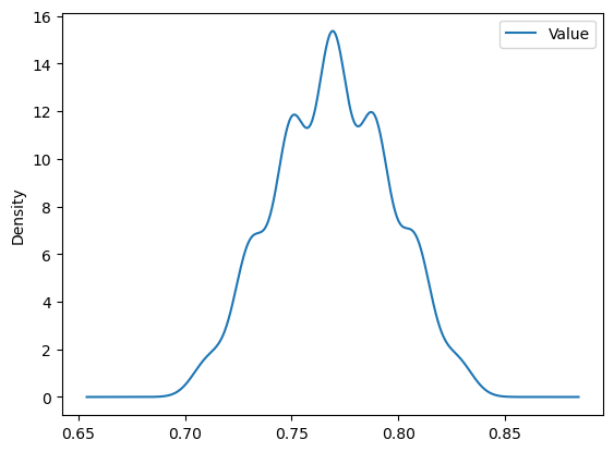
For example, if we want to display the distribution of accuracy we can execute the follwoing code.
aux = pd.concat(mcm_bootstrap)
aux\
    .query('Metric == "Accuracy"')\
    .plot(kind = 'density', label = 'Accuracy')
plt.show()

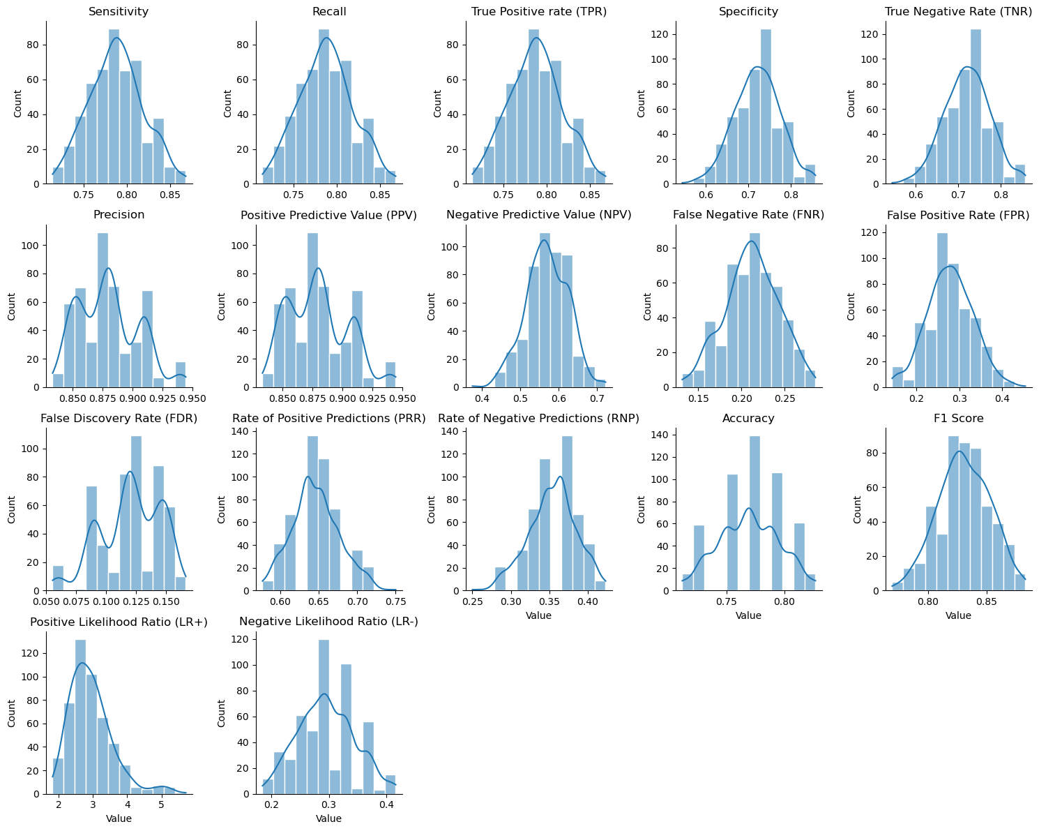
With seaborn is easy to display the distribution of all metrics.
g = sns.FacetGrid(pd.concat(mcm_bootstrap),
                  col = 'Metric',
                  col_wrap = 5,
                  sharey = False,
                  sharex = False)
g = g.map(sns.histplot, 'Value', bins = 12, kde = True, ec = 'white', )
g = g.set_titles('{col_name}', size = 12)

The mcm function can help us to analyse a confusion matrix. If this confusion matrix come from a performed model, we can evaluate it with this function: Sensitivity and Specificity as principal metrics.
pylint
$ pylint mcm.py --good-names=tn,fp,fn,tp
--------------------------------------------------------------------
Your code has been rated at 10.00/10 (previous run: 10.00/10, +0.00)


